Machine Learning Basics

🤖 Welcome to Machine Learning: Teaching Computers to Learn!

Today we’re diving into the amazing world of Machine Learning - where we teach computers to recognize patterns and make predictions, just like you learn from experience! 🧠✨

The Big Idea: Instead of programming every rule manually, we show the computer examples and let it figure out the patterns on its own. Mind-blowing, right?

Part 1: How Does Learning Work? 🤔

Let’s Think Like a Learner First!

Before we teach a computer, let’s understand how you learn by looking at movie posters!

Patterns Observed by Humans: Film Posters 🎬

Imagine: You’re at a movie theater and you see posters for films about the action-packed duo, Smiles and Smiley and their adventures. Your job is to spot the pattern!

The Training Set: Learn from These!

Let’s look at four movie posters and train our brains to recognize the pattern:

Smiles and Smiley in Space! logo

Smiles and Smiley Go West! logo

Smiles and Smiley in the Mountains! logo

Smiles and Smiley at the Seashore! logo

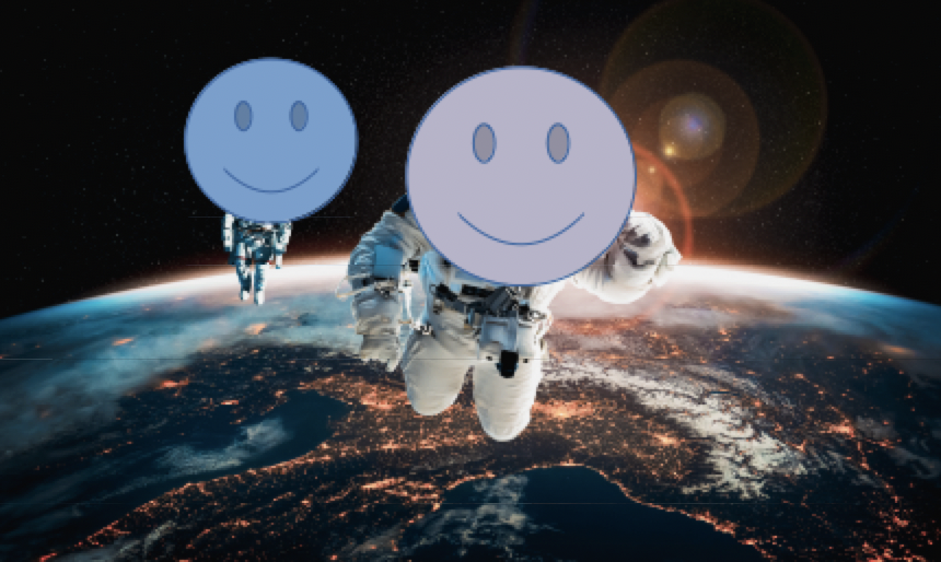
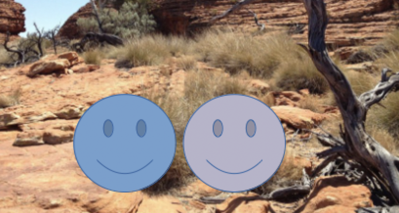
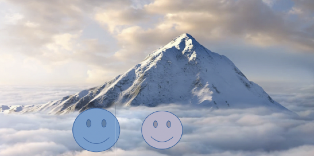
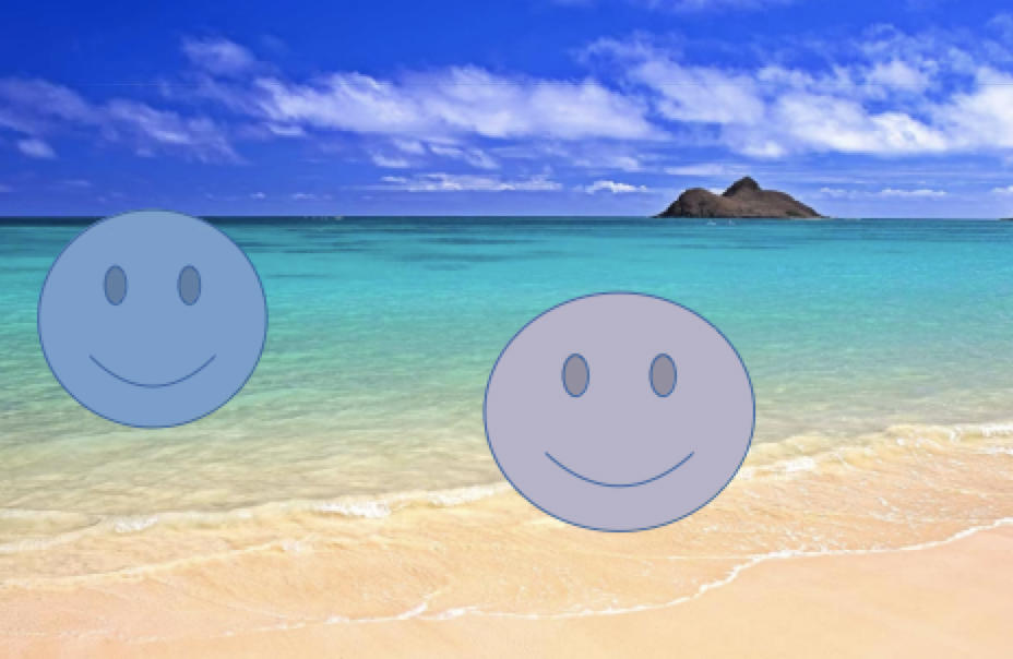
If you have studied these posters, then you have certainly noticed that there is a recognizable (and common) theme across all the posters of the set.

Can you spot the pattern? 🔍

The Test Case: What’s Different?

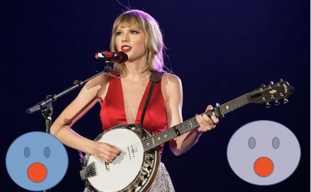
Now look at this NEW poster. Something’s different!

What common element of the above posters did you not see?
What is the common theme?!

One of the common features is that Smiles and Smiley were always featured in front of some beautiful and outdoors scene. In the last poster, Smiles and Smiley were featured singing with Taylor Swift.

Smiles and Smiley Sing with Swift! Smiles and Smiley with Taylor Swift

Detective Questions:

What common element is MISSING in this poster?
What pattern did the first four posters share?

🎯 The Answer: Outdoor Backgrounds!

The pattern: In the first four posters, Smiles and Smiley were always featured in front of beautiful outdoor scenes (space, desert, mountains, beach)!

In the Taylor Swift poster, they’re indoors at a concert - no outdoor background!

This is EXACTLY how machine learning works!

📖 Training: Show the computer examples (the first 4 posters)
🧠 Learning: Computer finds the common pattern (outdoor backgrounds)
✅ Testing: Show a new poster → Computer predicts if it fits the pattern!

Congratulations! You just learned like a machine learning algorithm! Your brain:

Observed training examples
Identified the pattern
Made a prediction about new data

Now let’s see how computers do the same thing with code! 🚀

Part 2: The Three Types of Machine Learning 🧠

Just like there are different ways YOU learn (from a teacher, by exploring, by trial and error), machines can learn in different ways too!

1️⃣ Supervised Learning: Learning with a Teacher 👩‍🏫

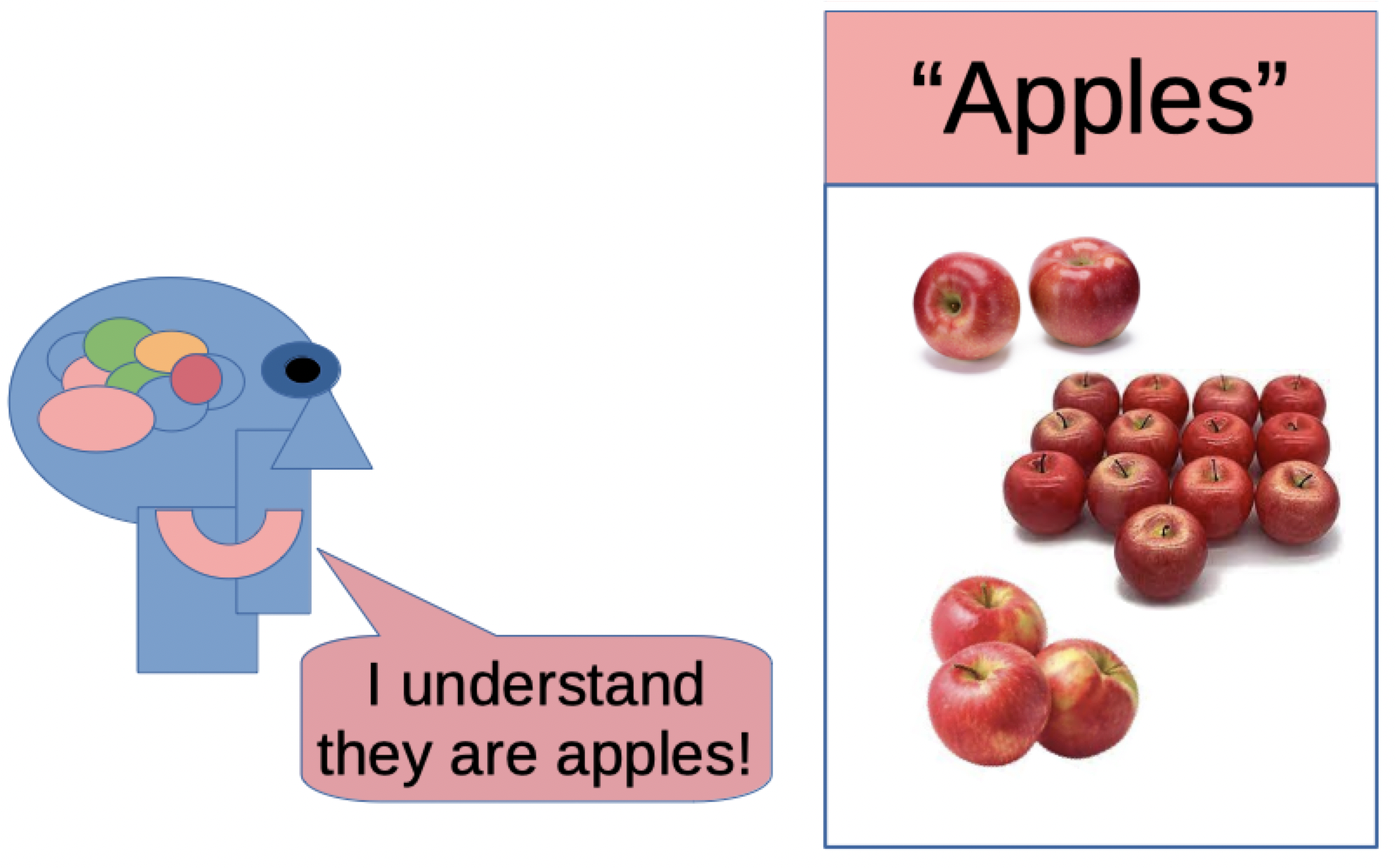
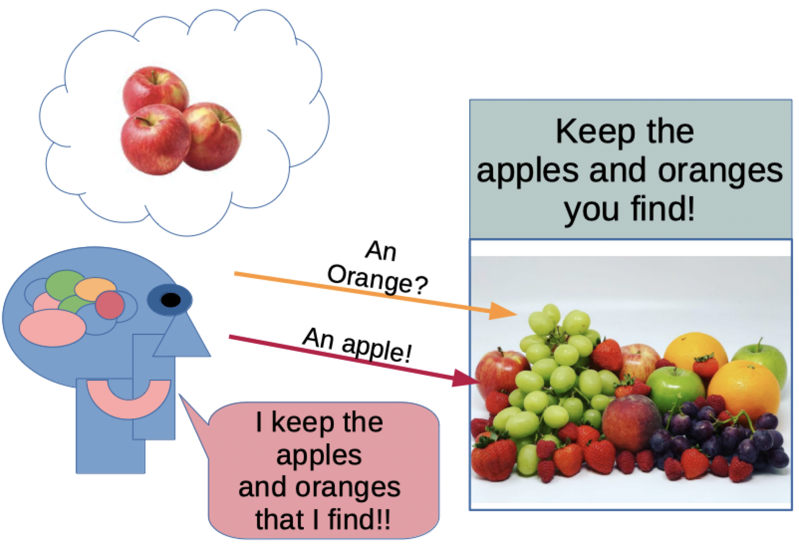
The Idea: The computer is shown examples WITH the correct answers (labels), like a teacher showing you flashcards!

Real-world example: Showing a computer 1000 pictures:

500 labeled “cat” 🐱
500 labeled “dog” 🐶

The computer learns: “Pointy ears + whiskers + small = cat” and “Floppy ears + bigger + tail wags = dog”

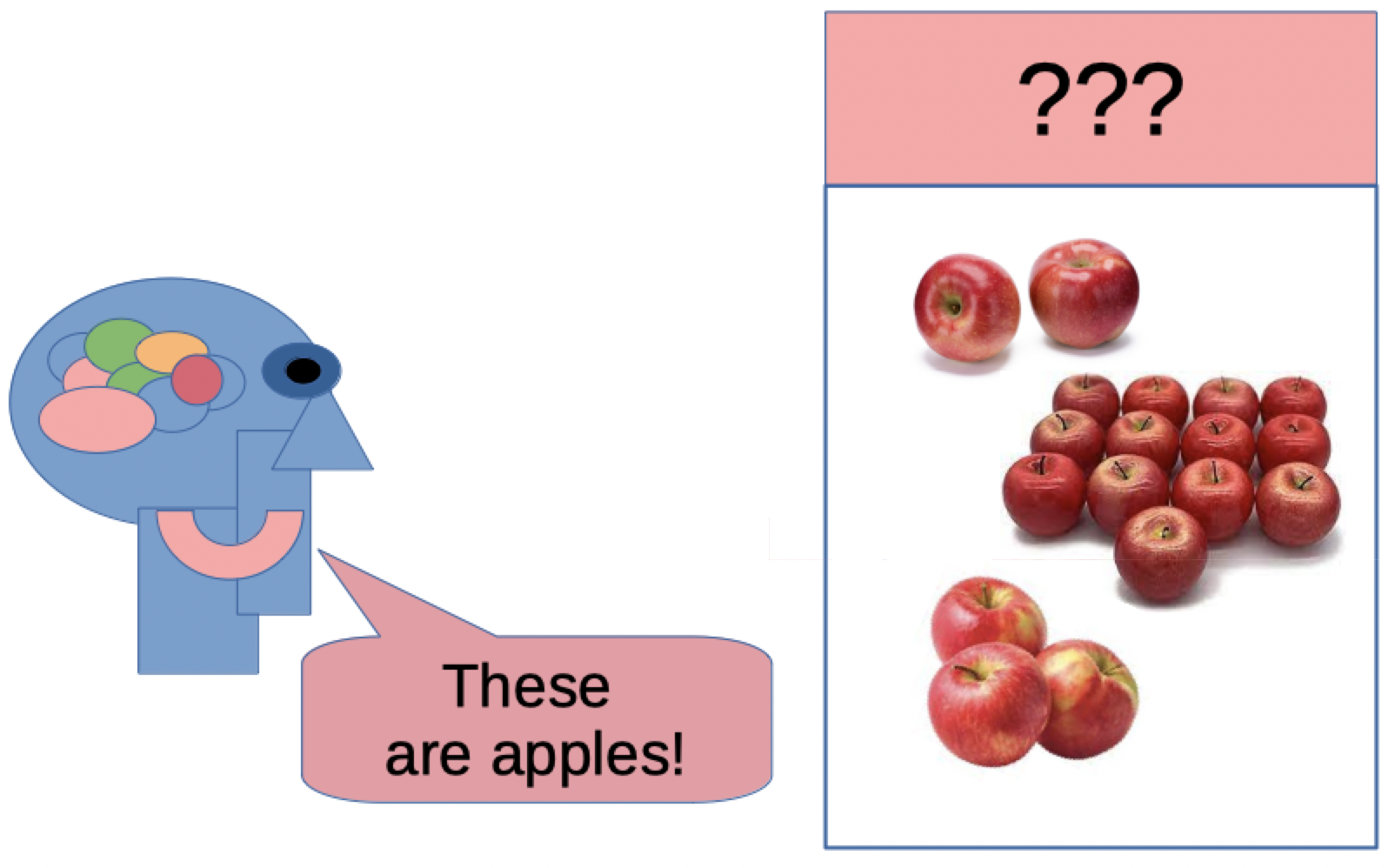
Then when you show it a NEW picture, it can predict: “That’s a cat!” or “That’s a dog!”

Where it’s used:

📧 Email spam detection (spam vs. not spam)
🏥 Medical diagnosis (disease vs. healthy)
💳 Credit card fraud detection (fraud vs. legitimate)
🌶️ Weather prediction (temperature tomorrow)
🚗 Self-driving cars (stop sign vs. speed limit sign)

Visual Example: Supervised Learning

Learning Task:

Recognition Task:

2️⃣ Unsupervised Learning: Exploring on Your Own 🔍

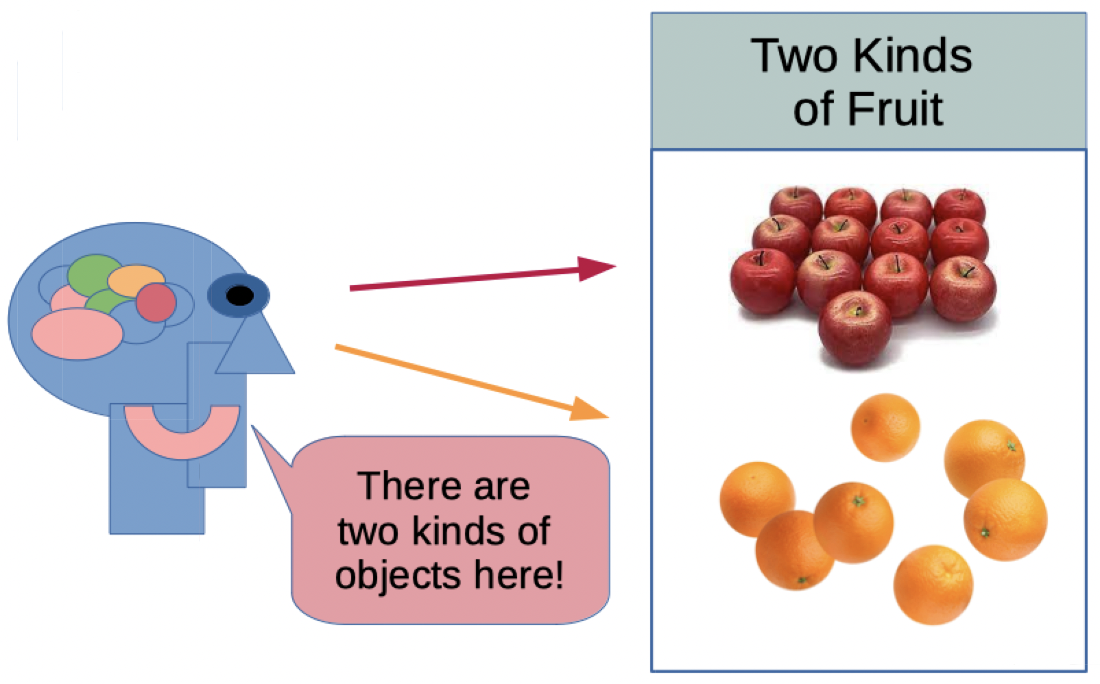
The Idea: NO labels, NO teacher! The computer explores the data and finds hidden patterns all by itself!

Real-world analogy: Imagine you have a box of 1000 buttons 🔘 of different colors, sizes, and shapes. Without anyone telling you, you naturally start grouping them:

All red ones together
All big ones together
All star-shaped ones together

That’s unsupervised learning! Finding groups (clusters) without being told what to look for.

Where it’s used:

🛒 Customer segmentation (grouping shoppers by behavior)
📰 News article grouping (topics that naturally emerge)
🧬 Gene analysis (finding patterns in DNA)
🎵 Music recommendation (songs that “go together”)
🤖 Anomaly detection (finding weird outliers)

3️⃣ Reinforcement Learning: Learning by Trial and Error 🎮

The Idea: The computer learns by DOING! It tries actions, gets rewards (good!) or penalties (bad!), and learns what works best.

Real-world analogy: Training a dog! 🐕

Dog sits → Gets treat → Learns sitting is good!
Dog jumps on couch → No treat (or timeout) → Learns jumping is bad!

Like playing a video game:

Move right → Collect coin (+10 points) ✅
Fall in pit → Lose life (-50 points) ❌
Defeat boss → Win game (+1000 points) 🏆

The computer tries MILLIONS of times, learning what actions lead to the best rewards!

Where it’s used:

🎮 Game AI (AlphaGo beating world champions!)
🚗 Self-driving cars (learning to navigate traffic)
🤖 Robot control (learning to walk, grasp objects)
💹 Stock trading bots (learning when to buy/sell)
🏭 Factory optimization (learning efficient workflows)

The learning cycle:

👀 Observe the current situation (state)
🎯 Take an action
🎁 Get a reward (or penalty)
🧠 Learn: “Was that good or bad?”
🔄 Repeat millions of times!

Part 3: Let’s Code! Hands-On ML Projects 💻

Time to get your hands dirty with REAL machine learning code! Each example includes detailed explanations so you understand exactly what’s happening.

Project 1: Supervised Learning - Classifying Flowers 🌸

The Goal: Train a computer to identify different types of iris flowers based on their measurements!

Dataset: The famous Iris dataset (3 flower species, 4 measurements each)

import numpy as np
import matplotlib.pyplot as plt
from sklearn.datasets import load_iris
from sklearn.model_selection import train_test_split
from sklearn.neighbors import KNeighborsClassifier
from sklearn.metrics import accuracy_score, confusion_matrix
import seaborn as sns

# Load the Iris dataset
iris = load_iris()
X = iris.data  # Features: sepal length, sepal width, petal length, petal width
y = iris.target  # Labels: 0=setosa, 1=versicolor, 2=virginica

print("🌸 IRIS FLOWER CLASSIFICATION")
print("=" * 60)
print(f"Total samples: {len(X)}")
print(f"Features per flower: {X.shape[1]}")
print(f"Classes: {iris.target_names}")
print("\nFirst 5 flowers:")
for i in range(5):
    print(f"  Flower {i+1}: {X[i]} → {iris.target_names[y[i]]}")

# Split into training (80%) and testing (20%) sets
X_train, X_test, y_train, y_test = train_test_split(
    X, y, test_size=0.2, random_state=42
)

print(f"\n📊 Data split:")
print(f"  Training samples: {len(X_train)}")
print(f"  Testing samples: {len(X_test)}")

# Create and train the model
# K-Nearest Neighbors: predicts based on the 5 closest training examples
model = KNeighborsClassifier(n_neighbors=5)
model.fit(X_train, y_train)

print("\n🎓 Training complete!")

# Make predictions on test data
y_pred = model.predict(X_test)

# Calculate accuracy
accuracy = accuracy_score(y_test, y_pred)

print(f"\n✅ Model accuracy: {accuracy * 100:.1f}%")
print(f"   Got {int(accuracy * len(y_test))} out of {len(y_test)} correct!")

# Show some predictions
print("\n🔮 Sample predictions:")
for i in range(5):
    actual = iris.target_names[y_test[i]]
    predicted = iris.target_names[y_pred[i]]
    match = "✅" if actual == predicted else "❌"
    print(f"   {match} Actual: {actual:12} | Predicted: {predicted}")

# Visualize the confusion matrix
cm = confusion_matrix(y_test, y_pred)
plt.figure(figsize=(8, 6))
sns.heatmap(cm, annot=True, fmt='d', cmap='Blues', 
            xticklabels=iris.target_names,
            yticklabels=iris.target_names)
plt.title('Confusion Matrix: How Well Did We Do?', fontsize=14, fontweight='bold')
plt.ylabel('Actual Species')
plt.xlabel('Predicted Species')
plt.tight_layout()
plt.show()

# Test with a NEW flower
new_flower = [[5.1, 3.5, 1.4, 0.2]]  # Example measurements
prediction = model.predict(new_flower)
print(f"\n🌺 New flower prediction: {iris.target_names[prediction[0]]}")

What’s happening:

Load Data: Get 150 iris flower measurements
Split Data: 80% for training, 20% for testing (never seen by model!)
Train: Model learns patterns from training data
Predict: Model guesses flower types for test data
Evaluate: Check accuracy - how many did we get right?

The Math Behind It:

K-Nearest Neighbors (KNN):

When predicting a new flower, it looks at the 5 most similar flowers it’s seen before
“Birds of a feather flock together” - similar flowers are probably the same species!
Distance formula: √[(x₁-x₂)² + (y₁-y₂)² + …]

Try this:

Change n_neighbors from 5 to 1, 3, or 10 - what happens to accuracy?
Predict your own flower: new_flower = [[6.0, 3.0, 4.0, 1.2]]

Project 2: Unsupervised Learning - Customer Segmentation 🛒

The Goal: Group customers into similar clusters WITHOUT being told what the groups are!

import numpy as np
import matplotlib.pyplot as plt
from sklearn.cluster import KMeans
from sklearn.preprocessing import StandardScaler

# Simulated customer data: age and annual spending
np.random.seed(42)

# Group 1: Young, low spenders
group1_age = np.random.normal(25, 5, 50)
group1_spending = np.random.normal(20000, 5000, 50)

# Group 2: Middle-aged, high spenders
group2_age = np.random.normal(45, 5, 50)
group2_spending = np.random.normal(60000, 10000, 50)

# Group 3: Seniors, moderate spenders
group3_age = np.random.normal(65, 5, 50)
group3_spending = np.random.normal(35000, 7000, 50)

# Combine all customers
ages = np.concatenate([group1_age, group2_age, group3_age])
spending = np.concatenate([group1_spending, group2_spending, group3_spending])
X = np.column_stack([ages, spending])

print("🛒 CUSTOMER SEGMENTATION (Unsupervised Learning)")
print("=" * 60)
print(f"Total customers: {len(X)}")
print(f"Features: Age, Annual Spending")
print("\nRemember: We're NOT telling the algorithm about the 3 groups!")
print("It will discover them on its own! 🔍\n")

# Standardize features (make them comparable)
scaler = StandardScaler()
X_scaled = scaler.fit_transform(X)

# Try different numbers of clusters
print("🧪 Testing different cluster counts...")
for n_clusters in [2, 3, 4, 5]:
    kmeans = KMeans(n_clusters=n_clusters, random_state=42, n_init=10)
    labels = kmeans.fit_predict(X_scaled)
    
    # Inertia = how tight the clusters are (lower is better)
    inertia = kmeans.inertia_
    print(f"  {n_clusters} clusters: inertia = {inertia:.2f}")

# Use 3 clusters (we happen to know there are 3 groups!)
kmeans = KMeans(n_clusters=3, random_state=42, n_init=10)
labels = kmeans.fit_predict(X_scaled)
centers = scaler.inverse_transform(kmeans.cluster_centers_)

print(f"\n✅ Segmented into 3 customer groups!")
print("\n📊 Cluster Centers (Average Customer in Each Group):")
for i, center in enumerate(centers):
    count = np.sum(labels == i)
    print(f"  Group {i+1}: Age={center[0]:.1f}, Spending=${center[1]:,.0f} ({count} customers)")

# Visualize the clusters
plt.figure(figsize=(12, 5))

# Before clustering
plt.subplot(1, 2, 1)
plt.scatter(ages, spending, alpha=0.6, s=100, c='gray', edgecolors='black')
plt.xlabel('Age', fontsize=12)
plt.ylabel('Annual Spending ($)', fontsize=12)
plt.title('Before Clustering\n(All customers look the same)', fontsize=14, fontweight='bold')
plt.grid(alpha=0.3)

# After clustering
plt.subplot(1, 2, 2)
colors = ['#FF6B6B', '#4ECDC4', '#FFE66D']
for i in range(3):
    cluster_points = X[labels == i]
    plt.scatter(cluster_points[:, 0], cluster_points[:, 1], 
                alpha=0.6, s=100, c=colors[i], edgecolors='black',
                label=f'Group {i+1}')

# Plot cluster centers
plt.scatter(centers[:, 0], centers[:, 1], 
            s=500, c='red', marker='*', 
            edgecolors='black', linewidth=2,
            label='Cluster Centers', zorder=5)

plt.xlabel('Age', fontsize=12)
plt.ylabel('Annual Spending ($)', fontsize=12)
plt.title('After Clustering\n(3 distinct customer segments!)', fontsize=14, fontweight='bold')
plt.legend()
plt.grid(alpha=0.3)

plt.tight_layout()
plt.show()

# Predict cluster for a new customer
new_customer = [[35, 45000]]  # 35 years old, spends $45k/year
new_customer_scaled = scaler.transform(new_customer)
cluster = kmeans.predict(new_customer_scaled)[0]
print(f"\n🎯 New customer (age 35, spending $45k) belongs to Group {cluster + 1}")

What’s happening:

Generate Data: Create 150 fake customers (but we don’t label them!)
Standardize: Make age and spending comparable (both on same scale)
Cluster: Algorithm finds 3 natural groups automatically!
Analyze: Look at each group’s characteristics

The Math Behind It:

K-Means Clustering:

Randomly place 3 “center points”
Assign each customer to nearest center
Move centers to the middle of their assigned customers
Repeat steps 2-3 until centers stop moving!

Distance formula: √[(age₁ - age₂)² + (spending₁ - spending₂)²]

Try this:

Change to 4 or 5 clusters - does it still make sense?
Add your own customer: [[50, 70000]] - which group do they join?

Project 3: Reinforcement Learning - Treasure Hunt! 💎

The Goal: Teach an agent to find treasure in a grid world by learning from rewards!

The Setup:

5×5 grid world
Agent starts at position (0, 0)
Treasure at position (4, 4)
Agent learns: Which moves lead to treasure?

import numpy as np
import matplotlib.pyplot as plt
from matplotlib.patches import Rectangle

# Create the environment
GRID_SIZE = 5
TREASURE_POS = (4, 4)
START_POS = (0, 0)

# Q-table: stores "quality" of each action at each position
# Actions: 0=up, 1=down, 2=left, 3=right
q_table = np.zeros((GRID_SIZE, GRID_SIZE, 4))

# Learning parameters
LEARNING_RATE = 0.1  # How quickly we update our knowledge
DISCOUNT = 0.95  # How much we care about future rewards
EPISODES = 500  # Number of times to practice
EPSILON = 0.1  # 10% chance to explore randomly

# Move deltas: [up, down, left, right]
MOVES = [(-1, 0), (1, 0), (0, -1), (0, 1)]
MOVE_NAMES = ['Up', 'Down', 'Left', 'Right']

def get_reward(position):
    """Return reward for reaching this position"""
    if position == TREASURE_POS:
        return 100  # Found treasure! 💎
    return -1  # Small penalty for each step (encourages efficiency)

def move(position, action):
    """Try to move in the chosen direction"""
    new_pos = (
        position[0] + MOVES[action][0],
        position[1] + MOVES[action][1]
    )
    
    # Check if move is valid (stay in bounds)
    if 0 <= new_pos[0] < GRID_SIZE and 0 <= new_pos[1] < GRID_SIZE:
        return new_pos
    return position  # Hit wall, stay in place

print("💎 REINFORCEMENT LEARNING: TREASURE HUNT")
print("=" * 60)
print(f"Grid size: {GRID_SIZE}×{GRID_SIZE}")
print(f"Start: {START_POS}, Treasure: {TREASURE_POS}")
print(f"Training episodes: {EPISODES}\n")

# Track learning progress
episode_rewards = []
episode_lengths = []

# Training loop
for episode in range(EPISODES):
    position = START_POS
    total_reward = 0
    steps = 0
    
    while position != TREASURE_POS and steps < 50:  # Max 50 steps per episode
        # Choose action: explore vs exploit
        if np.random.random() < EPSILON:
            action = np.random.randint(4)  # Random exploration
        else:
            action = np.argmax(q_table[position[0], position[1]])  # Use learned knowledge
        
        # Take action
        new_position = move(position, action)
        reward = get_reward(new_position)
        
        # Q-Learning update formula
        # New Q = Old Q + α × [Reward + γ × MaxFutureQ - Old Q]
        old_q = q_table[position[0], position[1], action]
        max_future_q = np.max(q_table[new_position[0], new_position[1]])
        new_q = old_q + LEARNING_RATE * (reward + DISCOUNT * max_future_q - old_q)
        q_table[position[0], position[1], action] = new_q
        
        position = new_position
        total_reward += reward
        steps += 1
    
    episode_rewards.append(total_reward)
    episode_lengths.append(steps)
    
    if (episode + 1) % 100 == 0:
        avg_reward = np.mean(episode_rewards[-100:])
        avg_steps = np.mean(episode_lengths[-100:])
        print(f"Episode {episode + 1}: Avg reward = {avg_reward:.1f}, Avg steps = {avg_steps:.1f}")

print("\n✅ Training complete!\n")

# Test the learned policy
print("🎯 Testing learned path:")
position = START_POS
path = [position]
steps = 0

while position != TREASURE_POS and steps < 20:
    action = np.argmax(q_table[position[0], position[1]])
    position = move(position, action)
    path.append(position)
    steps += 1
    print(f"  Step {steps}: Move {MOVE_NAMES[action]} → Position {position}")

print(f"\n🏆 Found treasure in {steps} steps!")

# Visualize the learned path
fig, (ax1, ax2, ax3) = plt.subplots(1, 3, figsize=(18, 6))

# Plot 1: Learning progress
ax1.plot(episode_rewards, alpha=0.3, color='blue')
window = 50
smoothed = np.convolve(episode_rewards, np.ones(window)/window, mode='valid')
ax1.plot(smoothed, color='red', linewidth=2, label=f'{window}-episode average')
ax1.set_xlabel('Episode', fontsize=12)
ax1.set_ylabel('Total Reward', fontsize=12)
ax1.set_title('Learning Progress Over Time', fontsize=14, fontweight='bold')
ax1.legend()
ax1.grid(alpha=0.3)

# Plot 2: Grid with learned path
ax2.set_xlim(-0.5, GRID_SIZE - 0.5)
ax2.set_ylim(-0.5, GRID_SIZE - 0.5)
ax2.set_aspect('equal')
ax2.invert_yaxis()  # Make (0,0) at top-left

# Draw grid
for i in range(GRID_SIZE):
    for j in range(GRID_SIZE):
        rect = Rectangle((j-0.5, i-0.5), 1, 1, 
                         fill=True, facecolor='lightgray', 
                         edgecolor='black', linewidth=2)
        ax2.add_patch(rect)

# Draw path
for i in range(len(path) - 1):
    y1, x1 = path[i]
    y2, x2 = path[i + 1]
    ax2.arrow(x1, y1, x2-x1, y2-y1, 
              head_width=0.2, head_length=0.1,
              fc='blue', ec='blue', linewidth=3, alpha=0.7)

# Mark start and treasure
ax2.text(START_POS[1], START_POS[0], '🚀', 
         fontsize=30, ha='center', va='center')
ax2.text(TREASURE_POS[1], TREASURE_POS[0], '💎', 
         fontsize=30, ha='center', va='center')

ax2.set_xticks(range(GRID_SIZE))
ax2.set_yticks(range(GRID_SIZE))
ax2.set_title(f'Learned Path ({len(path)-1} steps)', fontsize=14, fontweight='bold')
ax2.grid(True, alpha=0.3)

# Plot 3: Q-values heatmap (best action at each position)
best_actions = np.argmax(q_table, axis=2)
ax3.imshow(best_actions, cmap='viridis', alpha=0.3)

# Draw arrows showing best action at each position
for i in range(GRID_SIZE):
    for j in range(GRID_SIZE):
        if (i, j) == TREASURE_POS:
            ax3.text(j, i, '💎', fontsize=25, ha='center', va='center')
        else:
            best_action = best_actions[i, j]
            arrows = ['↑', '↓', '←', '→']
            ax3.text(j, i, arrows[best_action], 
                    fontsize=20, ha='center', va='center', 
                    fontweight='bold', color='blue')

ax3.set_xticks(range(GRID_SIZE))
ax3.set_yticks(range(GRID_SIZE))
ax3.set_title('Learned Policy\n(Best action at each position)', 
              fontsize=14, fontweight='bold')
ax3.grid(True, alpha=0.3)

plt.tight_layout()
plt.show()

print("\n💡 What the agent learned:")
print("   - Moving toward treasure = good (positive rewards)")
print("   - Each step costs energy (small penalty)")
print("   - Over time, found the OPTIMAL path!")
print("   - This is how robots learn to navigate! 🤖")

What’s happening:

Q-Table: Stores learned value of each action at each position
Explore vs Exploit: Sometimes try random moves (explore), sometimes use best known move (exploit)
Rewards: +100 for treasure, -1 per step (encourages efficiency)
Update: After each move, update Q-table based on reward received
Improve: Over 500 episodes, agent learns optimal path!

The Math Behind It:

Q-Learning Update Formula:

New Q-value = Old Q-value + α × [Reward + γ × Max(Future Q-values) - Old Q-value]

Where:

α (alpha): Learning rate (0.1) - how much to update each step
γ (gamma): Discount factor (0.95) - how much to value future rewards
Reward: Immediate reward from action
Max(Future Q-values): Best possible value from next position

Try this:

Change treasure position: TREASURE_POS = (2, 3)
Add obstacles (walls) to make it harder
Increase grid size: GRID_SIZE = 10
Try different learning rates: LEARNING_RATE = 0.5

Part 4: Comparing the Three Types 📊

Type	Supervised	Unsupervised	Reinforcement
Training Data	Labeled (with answers)	Unlabeled (no answers)	Trial & error
Goal	Predict correct answer	Find hidden patterns	Maximize rewards
Example	Email spam filter	Customer grouping	Game playing AI
Like…	Learning with flashcards	Organizing your closet	Learning to ride a bike
Feedback	Teacher tells you if correct	No external feedback	Rewards/penalties

Conclusion: You’re Now an ML Programmer! 🎓

What You’ve Accomplished:

✅ Understood how machines learn (like humans!)
✅ Explored all 3 types of machine learning
✅ Coded real ML projects:

Supervised: Flower classification
Unsupervised: Customer segmentation
Reinforcement: Treasure hunt agent
✅ Visualized how algorithms learn and make decisions

Key Takeaways:

Supervised Learning = Learning with a teacher (labeled data)
Unsupervised Learning = Finding patterns alone (no labels)
Reinforcement Learning = Learning by trial and error (rewards!)
More data = Better learning (usually!)
Visualization helps understand what’s happening

Your Next Steps 🚀

Challenge Projects:

Image Classifier: Train a model to recognize handwritten digits (MNIST dataset)
Movie Recommender: Use clustering to group similar movies
Snake Game AI: Use RL to teach an agent to play Snake!

Keep Learning! 📚

Online Resources:

Specific Topics:

Advanced Adventures:

Neural Networks: The brain-inspired approach to ML
Deep Learning: Neural networks with many layers (recognizing cats, faces, voices!)
Computer Vision: Teaching computers to “see” and understand images
Natural Language Processing: Teaching computers to understand human language

Final Thoughts 💭

Machine learning is transforming our world:

📱 Your phone’s face unlock
🎵 Spotify recommendations
🚗 Self-driving cars
🏥 Disease diagnosis
🎮 Video game AI

You now have the foundation to build the next generation of AI! Keep experimenting, keep learning, and most importantly - have fun building intelligent systems! 🤖✨

Remember: Every ML expert started exactly where you are now. The only difference? They kept coding, kept learning, and never gave up. You can do this! 💪🚀

I, Oliver Bonham-Carter 👋

Associate Professor in The Department of Computer and Information Science, Allegheny College

I, Oliver Bonham-Carter 👋

Associate Professor in The Department of Computer and Information Science, Allegheny College

Machine Learning Basics

🤖 Welcome to Machine Learning: Teaching Computers to Learn!

Part 1: How Does Learning Work? 🤔

Let’s Think Like a Learner First!

Patterns Observed by Humans: Film Posters 🎬

The Training Set: Learn from These!

The Test Case: What’s Different?

🎯 The Answer: Outdoor Backgrounds!

Part 2: The Three Types of Machine Learning 🧠

1️⃣ Supervised Learning: Learning with a Teacher 👩‍🏫

Visual Example: Supervised Learning

2️⃣ Unsupervised Learning: Exploring on Your Own 🔍

3️⃣ Reinforcement Learning: Learning by Trial and Error 🎮

Part 3: Let’s Code! Hands-On ML Projects 💻

Project 1: Supervised Learning - Classifying Flowers 🌸

Project 2: Unsupervised Learning - Customer Segmentation 🛒

Project 3: Reinforcement Learning - Treasure Hunt! 💎

Part 4: Comparing the Three Types 📊

Conclusion: You’re Now an ML Programmer! 🎓

What You’ve Accomplished:

Key Takeaways:

Your Next Steps 🚀

Keep Learning! 📚

Final Thoughts 💭